In this notebook, we will attempt to rebuild our MNIST digit classifier using convolutions in our neural network.
This notebook is based on the Fast AI book’s chapter 13 on convolutions (link).
Convolutional Neural Networks
Convolution
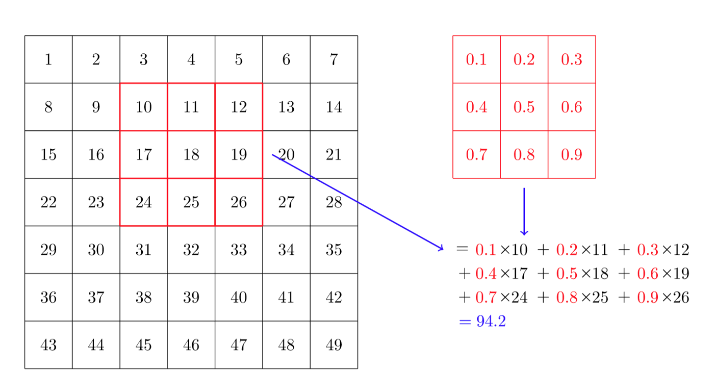
Convolutions allow us to distinguish important features in our images more readily. The way that they operate is by applying a filter kernel across our image.
This following image provides another view of what is happening in our convolutional neural network:
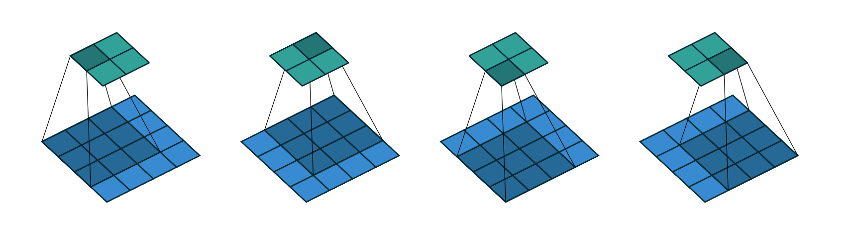
As we can see, each convolution allows us to hone in on more specific features of our image. For example, some of our kernels will detect horizontal edges, vertical edges, or diagonal edges. These help classify objects like digits more precisely.
In Pytorch, these convolutions can be easily implemented using the following functional F.conv2d or using the class nn.Conv2d. These take in rank 4 tensors of the form [batch_size, channels, width, height].
Quick Note: In numerical image procesing, a channel refers to the color scale of our image. Hence, for a grayscale image, we have 1 channel. For a RGB image, we have 3 channels. Convolutions can deal with any number of channels.
Our weights are kernels of shape (out_cannels, in_channels, kH, kW).
There is a formula that is useful for this type of operations. Given a image and a filter, kernel of shape we get the following equation for the shape of our activaton feature map .
Paddings and Strides
As we see from the previous section, our feature map will be reduced. With multiple layers of convolutions, we get smaller and smaller feature maps. In order to maintain the same size as our input, we need to satisfy the following equation .
Padding helps us make our input bigger by adding extra space around our input (usually with value 0). This allows us to keep a bigger feature map.
For an odd shaped kernel, the equation for maintaining feature map shape is .
Strides tell us how many pixels to jump over when applying the filter kernel over our input image. Striding tells us how many low-level features are ignored. With a stride-2 convolution, we decrease the activation map by a factor of 4. We thus want to increase the number of ouput activations to make sure that we don’t decrease the capacity of a layer by too much. It halves the width and height of each input. Doubling the number of filters does not change the overall amount of computation. It allows us to extract richer features with each successive layer.
Batch Normalization
This is a technique by converting the activations of a layer into standard units. It also adds two learnable parameters (usually called gamma [] and beta[]) that help account for activation differentiation (ie when you want some activations to be really high in order to make accurate predictions). The normalizing process yields an activation vector and return .
This helps improve the accuracy of our models.
MNIST Digit Classifier
Exploration
This is the same dataset that we used for our old MNIST digit classifier dataset. We are applying the same image transformations to normalize them.
import torch
import torch.nn as nn
import torch.nn.functional as F
from torch.utils.data import DataLoader, random_split, Dataset

import torchvision
from torchvision.transforms import v2
import torchvision.models as models

import numpy as np
#normalization functions for our dataset
transformations = v2.Compose([v2.ToImage(), v2.ToDtype(torch.float32, scale = True), v2.Normalize((0.1307,), (0.3081,))])
train_ds = torchvision.datasets.MNIST(
root = ".", train = True, download = True, transform = transformations
)
test_ds = torchvision.datasets.MNIST(
root = ".", train = False, download = True, transform = transformations
)
print(f"The length of our training dataset: {len(train_ds)}")
v2.ToPILImage()(train_ds[0][0]).resize((100,100))The length of our training dataset: 60000
<PIL.Image.Image image mode=L size=100x100>A great way to improve the accuracy of our model is by increasing our batch size. It’s important to be careful when choosing our batch size as the bigger the batch size, the more memory it takes.
It is also important to make sure that our batch size is reasonable with respect to the size of the full dataset. Here, since we have 60,000 images in our dataset, we can work with a batchsize of 512.
valid_size = int(0.1 * len(train_ds))
train_size = len(train_ds) - valid_size

train_ds, valid_ds = random_split(train_ds, [train_size, valid_size])

train_dl = DataLoader(train_ds, batch_size = 512, shuffle = True)
valid_dl = DataLoader(train_ds, batch_size = 512, shuffle = True)
xb, yb = next(iter(train_dl))
xb.shape, yb.shape(torch.Size([512, 1, 28, 28]), torch.Size([512]))Building our Model
#Choosing our device for acceleration
if torch.cuda.is_available(): #For NVIDIA GPU
    device = torch.device("cuda")
elif torch.backends.mps.is_available(): #For MAC OS
    device = torch.device("mps")
else:
    device = torch.device("cpu")

print(device)mpsIn code
def conv(ni, nf, ks = 3, act = True):
    layers = [nn.Conv2d(ni, nf, kernel_size = ks, padding = ks//2, stride = 2)]
    if act:
       layers.append(nn.ReLU())
    layers.append(nn.BatchNorm2d(nf))
    return nn.Sequential(*layers)

simple_cnn = nn.Sequential(
    conv(1, 4),
    conv(4, 8),
    conv(8,16),
    conv(16,32),
    conv(32, 64),
    conv(64, 10, act = False),
    nn.Flatten()
)

simple_nn = nn.Sequential(
    nn.Flatten(),
    nn.Linear(28*28, 128),
    nn.ReLU(),
    nn.Linear(128, 10)
)

loss_f = F.cross_entropy

print(simple_cnn(xb).shape)
simple_cnn.to(device), simple_nn.to(device)
torch.Size([512, 10])(Sequential(
(0): Sequential(
(0): Conv2d(1, 4, kernel_size=(3, 3), stride=(2, 2), padding=(1, 1))
(1): ReLU()
(2): BatchNorm2d(4, eps=1e-05, momentum=0.1, affine=True, track_running_stats=True)
)
(1): Sequential(
(0): Conv2d(4, 8, kernel_size=(3, 3), stride=(2, 2), padding=(1, 1))
(1): ReLU()
(2): BatchNorm2d(8, eps=1e-05, momentum=0.1, affine=True, track_running_stats=True)
)
(2): Sequential(
(0): Conv2d(8, 16, kernel_size=(3, 3), stride=(2, 2), padding=(1, 1))
(1): ReLU()
(2): BatchNorm2d(16, eps=1e-05, momentum=0.1, affine=True, track_running_stats=True)
)
(3): Sequential(
(0): Conv2d(16, 32, kernel_size=(3, 3), stride=(2, 2), padding=(1, 1))
(1): ReLU()
(2): BatchNorm2d(32, eps=1e-05, momentum=0.1, affine=True, track_running_stats=True)
)
(4): Sequential(
(0): Conv2d(32, 64, kernel_size=(3, 3), stride=(2, 2), padding=(1, 1))
(1): ReLU()
(2): BatchNorm2d(64, eps=1e-05, momentum=0.1, affine=True, track_running_stats=True)
)
(5): Sequential(
(0): Conv2d(64, 10, kernel_size=(3, 3), stride=(2, 2), padding=(1, 1))
(1): BatchNorm2d(10, eps=1e-05, momentum=0.1, affine=True, track_running_stats=True)
)
(6): Flatten(start_dim=1, end_dim=-1)
),
Sequential(
(0): Flatten(start_dim=1, end_dim=-1)
(1): Linear(in_features=784, out_features=128, bias=True)
(2): ReLU()
(3): Linear(in_features=128, out_features=10, bias=True)
))Notes on the code
Training
Very simple training loop using a Stochastic Gradient Descent (SGD) algorithm.
def train(model, model_name, train_dl, valid_dl, epochs = 10, lr = 0.06, loss_f = loss_f, params = None, scheduler = None, momentum = 0):
    if not params:
        params = model.parameters()

    sgd = torch.optim.SGD(params, lr = lr, momentum = momentum)
    if scheduler:
        scheduler = scheduler(sgd)

    def train_epoch():
        epoch_loss = np.array([])
        for xb, yb in train_dl:
            xb, yb = xb.to(device), yb.to(device)
            loss = loss_f(model(xb), yb)
            epoch_loss = np.append(epoch_loss, loss.item())
            loss.backward()
            sgd.step()
            sgd.zero_grad()
        return epoch_loss.mean()

    def validate_epoch():
        valid_loss = np.array([])
        accuracy = np.array([])
        for xb, yb in valid_dl:
            xb, yb = xb.to(device), yb.to(device)
            with torch.no_grad():
                pred = model(xb)
                loss = loss_f(pred, yb)
                valid_loss = np.append(valid_loss, loss.item())
                pred = torch.softmax(pred, dim = 1)
                infered_prediction = torch.argmax(pred, dim = 1)
                accuracy = np.append(accuracy, torch.Tensor.cpu((infered_prediction == yb).float()).mean())
        return valid_loss.mean(), accuracy.mean()

    print(f"Model: {model_name}")
    for ep in range(epochs):
        epoch_loss = train_epoch()
        valid_loss, accuracy = validate_epoch()
        if scheduler:
            scheduler.step()
        print(f"Ep #{ep+1} | Train Mean Loss: {round(epoch_loss, 3)} | Valid Mean Loss: {round(valid_loss,3)} | Accuracy: {round(accuracy,3)}")

    print("\n") # for clean separation of logging data
train(simple_cnn, "CNN", train_dl, valid_dl)
train(simple_nn, 'NN', train_dl, valid_dl)Model: CNN
Ep #1 | Train Mean Loss: 0.62 | Valid Mean Loss: 0.317 | Accuracy: 0.951
Ep #2 | Train Mean Loss: 0.253 | Valid Mean Loss: 0.202 | Accuracy: 0.966
Ep #3 | Train Mean Loss: 0.177 | Valid Mean Loss: 0.15 | Accuracy: 0.973
Ep #4 | Train Mean Loss: 0.138 | Valid Mean Loss: 0.123 | Accuracy: 0.978
Ep #5 | Train Mean Loss: 0.114 | Valid Mean Loss: 0.109 | Accuracy: 0.978
Ep #6 | Train Mean Loss: 0.099 | Valid Mean Loss: 0.092 | Accuracy: 0.982
Ep #7 | Train Mean Loss: 0.087 | Valid Mean Loss: 0.092 | Accuracy: 0.98
Ep #8 | Train Mean Loss: 0.078 | Valid Mean Loss: 0.071 | Accuracy: 0.986
Ep #9 | Train Mean Loss: 0.07 | Valid Mean Loss: 0.068 | Accuracy: 0.986
Ep #10 | Train Mean Loss: 0.066 | Valid Mean Loss: 0.062 | Accuracy: 0.987
Model: NN
Ep #1 | Train Mean Loss: 0.681 | Valid Mean Loss: 0.367 | Accuracy: 0.897
Ep #2 | Train Mean Loss: 0.33 | Valid Mean Loss: 0.296 | Accuracy: 0.915
Ep #3 | Train Mean Loss: 0.281 | Valid Mean Loss: 0.263 | Accuracy: 0.925
Ep #4 | Train Mean Loss: 0.251 | Valid Mean Loss: 0.238 | Accuracy: 0.931
Ep #5 | Train Mean Loss: 0.228 | Valid Mean Loss: 0.216 | Accuracy: 0.939
Ep #6 | Train Mean Loss: 0.21 | Valid Mean Loss: 0.201 | Accuracy: 0.943
Ep #7 | Train Mean Loss: 0.194 | Valid Mean Loss: 0.184 | Accuracy: 0.948
Ep #8 | Train Mean Loss: 0.181 | Valid Mean Loss: 0.174 | Accuracy: 0.951
Ep #9 | Train Mean Loss: 0.17 | Valid Mean Loss: 0.163 | Accuracy: 0.954
Ep #10 | Train Mean Loss: 0.159 | Valid Mean Loss: 0.153 | Accuracy: 0.957Testing
test_dl = DataLoader(test_ds, batch_size = 256, shuffle = True)

def test(model, test_dl):
    test_loss = np.array([])
    accuracy = np.array([])

    for xb, yb in test_dl:
        xb, yb = xb.to(device), yb.to(device)
        with torch.no_grad():
            pred = model(xb)
            loss = loss_f(pred, yb)
            test_loss = np.append(test_loss, loss.item())
            pred = torch.softmax(pred, dim = 1)
            infered_prediction = torch.argmax(pred, dim = 1)
            accuracy = np.append(accuracy, torch.Tensor.cpu((infered_prediction == yb).float()).mean())

    mean_accuracy = np.mean(accuracy)
    mean_loss = np.mean(test_loss)

    return mean_accuracy, mean_loss
cnn_test = test(simple_cnn, test_dl)
nn_test = test(simple_nn, test_dl)
print(f"We observe the following stats for our CNN: \nAccuracy: {cnn_test[0]} || Loss: {cnn_test[1]}")
print("\n")
print(f"We observe the following stats for our NN: \nAccuracy: {nn_test[0]} || Loss: {nn_test[1]}")We observe the following stats for our CNN:
Accuracy: 0.9765625 || Loss: 0.09848785679787397
We observe the following stats for our NN:
Accuracy: 0.95615234375 || Loss: 0.15647681355476378As we observe, our CNN is much more effective at recognizing our digits than the simple neural network.
Dog vs Cat Classifier
Exploration
from datasets import load_dataset

cats_dogs = load_dataset("microsoft/cats_vs_dogs")['train']display(cats_dogs['image'][0])
display(cats_dogs['image'][1])
<PIL.JpegImagePlugin.JpegImageFile image mode=RGB size=500x375>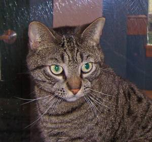
<PIL.JpegImagePlugin.JpegImageFile image mode=RGB size=300x281>transformation = v2.Compose([v2.Resize((128,128)),
v2.RandomHorizontalFlip(),
v2.RandomRotation(10),
v2.ColorJitter(brightness=0.1, contrast=0.1),
v2.Grayscale(num_output_channels = 3),
v2.ToImage(),
v2.ToDtype(torch.float32, scale = True),
])
class CatsDogsDataset(Dataset):
def __init__(self, images, labels, transform):
super().__init__()
self.data = images
self.labels = labels
self.transform = transform
def __len__(self):
return len(self.data)
def __getitem__(self, idx):
sample = self.data[idx]
label = self.labels[idx]
if self.transform:
sample = self.transform(sample)
return sample, label
cats_dogs_ds = CatsDogsDataset(cats_dogs['image'], cats_dogs['labels'], transformation)cats_dogs_ds[0](Image([[[0.0431, 0.0431, 0.0431, ..., 0.0431, 0.0431, 0.0431],
[0.0431, 0.0431, 0.0431, ..., 0.0431, 0.0431, 0.0431],
[0.0431, 0.0431, 0.0431, ..., 0.0431, 0.0431, 0.0431],
...,
[0.0431, 0.0431, 0.0431, ..., 0.0431, 0.0431, 0.0431],
[0.0431, 0.0431, 0.0431, ..., 0.0431, 0.0431, 0.0431],
[0.0431, 0.0431, 0.0431, ..., 0.0431, 0.0431, 0.0431]],
[[0.0431, 0.0431, 0.0431, ..., 0.0431, 0.0431, 0.0431],
[0.0431, 0.0431, 0.0431, ..., 0.0431, 0.0431, 0.0431],
[0.0431, 0.0431, 0.0431, ..., 0.0431, 0.0431, 0.0431],
...,
[0.0431, 0.0431, 0.0431, ..., 0.0431, 0.0431, 0.0431],
[0.0431, 0.0431, 0.0431, ..., 0.0431, 0.0431, 0.0431],
[0.0431, 0.0431, 0.0431, ..., 0.0431, 0.0431, 0.0431]],
[[0.0431, 0.0431, 0.0431, ..., 0.0431, 0.0431, 0.0431],
[0.0431, 0.0431, 0.0431, ..., 0.0431, 0.0431, 0.0431],
[0.0431, 0.0431, 0.0431, ..., 0.0431, 0.0431, 0.0431],
...,
[0.0431, 0.0431, 0.0431, ..., 0.0431, 0.0431, 0.0431],
[0.0431, 0.0431, 0.0431, ..., 0.0431, 0.0431, 0.0431],
[0.0431, 0.0431, 0.0431, ..., 0.0431, 0.0431, 0.0431]]], ),
0)len(cats_dogs_ds)23410test_split = int(len(cats_dogs_ds) * 0.2)
train_split = len(cats_dogs_ds) - test_split
train_valid_ds, test_ds = random_split(cats_dogs_ds, [test_split, train_split])
valid_split = int(len(train_valid_ds)*0.1)
train_split = len(train_valid_ds) - valid_split
train_ds, valid_ds = random_split(train_valid_ds, [valid_split, train_split])
train_dl = DataLoader(train_ds, batch_size = 512, shuffle = True)
valid_dl = DataLoader(valid_ds, batch_size = 512, shuffle = True )
test_dl = DataLoader(test_ds, batch_size = 512, shuffle = True)xb, yb = next(iter(train_dl))
xb.shape, yb.shape(torch.Size([468, 3, 128, 128]), torch.Size([468]))Our own model
cats_dogs_cnn = nn.Sequential(
                conv(3,6),
                conv(6, 12),
                conv(12, 24),
                conv(24, 48),
                nn.Dropout(p=0.5),
                conv(48, 96),
                conv(96, 192),
                conv(192, 384),
                conv(384, 2, act = False),
                nn.Flatten()
)

cats_dogs_cnn.to(device)
xb = xb.to(device)

cats_dogs_cnn(xb).shape
torch.Size([468, 2])train(cats_dogs_cnn, "Cats Dogs CNN", train_dl, valid_dl, epochs = 20)Model: Cats Dogs CNN
Ep #1 | Train Mean Loss: 0.873 | Valid Mean Loss: 0.876 | Accuracy: 0.515
Ep #2 | Train Mean Loss: 0.908 | Valid Mean Loss: 0.745 | Accuracy: 0.52
Ep #3 | Train Mean Loss: 0.698 | Valid Mean Loss: 0.705 | Accuracy: 0.545
Ep #4 | Train Mean Loss: 0.69 | Valid Mean Loss: 0.706 | Accuracy: 0.538
Ep #5 | Train Mean Loss: 0.691 | Valid Mean Loss: 0.705 | Accuracy: 0.536
Ep #6 | Train Mean Loss: 0.669 | Valid Mean Loss: 0.694 | Accuracy: 0.551
Ep #7 | Train Mean Loss: 0.674 | Valid Mean Loss: 0.706 | Accuracy: 0.531
Ep #8 | Train Mean Loss: 0.649 | Valid Mean Loss: 0.7 | Accuracy: 0.546
Ep #9 | Train Mean Loss: 0.664 | Valid Mean Loss: 0.705 | Accuracy: 0.536
Ep #10 | Train Mean Loss: 0.65 | Valid Mean Loss: 0.697 | Accuracy: 0.562
Ep #11 | Train Mean Loss: 0.668 | Valid Mean Loss: 0.699 | Accuracy: 0.546
Ep #12 | Train Mean Loss: 0.645 | Valid Mean Loss: 0.703 | Accuracy: 0.553
Ep #13 | Train Mean Loss: 0.632 | Valid Mean Loss: 0.698 | Accuracy: 0.559
Ep #14 | Train Mean Loss: 0.636 | Valid Mean Loss: 0.696 | Accuracy: 0.568
Ep #15 | Train Mean Loss: 0.648 | Valid Mean Loss: 0.694 | Accuracy: 0.573
Ep #16 | Train Mean Loss: 0.626 | Valid Mean Loss: 0.701 | Accuracy: 0.561
Ep #17 | Train Mean Loss: 0.633 | Valid Mean Loss: 0.71 | Accuracy: 0.562
Ep #18 | Train Mean Loss: 0.634 | Valid Mean Loss: 0.702 | Accuracy: 0.562
Ep #19 | Train Mean Loss: 0.619 | Valid Mean Loss: 0.705 | Accuracy: 0.562
Ep #20 | Train Mean Loss: 0.63 | Valid Mean Loss: 0.699 | Accuracy: 0.566accuracy, loss = test(cats_dogs_cnn, test_dl)
print(f"We find the following mean accuracy {accuracy} and loss {loss} for our model. ")We find the following mean accuracy 0.5662279145137684 and loss 0.6992067324148642 for our model.As we notice, this is not great accuracy. It seems that our model goes a little shy of guessing. Usually, it is rare to train a full CNN from scratch. We will now try a different approach: transfer learning!
Transfer Learning
For this task, we will use a Resnet 18!
It’s important to disable the gradient calculations for the parameters before the final layer so that we are not unnecessarily computing extra gradients. For this reason too, we will be only optimizing the parameters of our final layers.
Another important feature is that we are adding a learning rate scheduler.
resnet18 = models.resnet18(weights = "DEFAULT")
for param in resnet18.parameters():
    param.requires_grad = False

num_ftrs = resnet18.fc.in_features
resnet18.fc = nn.Sequential(
            nn.Linear(num_ftrs, 2),
)

resnet18.to(device)

steplr = lambda optim : torch.optim.lr_scheduler.StepLR(optim, step_size = 5, gamma = 0.1)

train(resnet18, "Resnet 18", train_dl, valid_dl, epochs = 25, params = resnet18.fc.parameters(), scheduler = steplr, lr = 0.06)
Model: Resnet 18
Ep #1 | Train Mean Loss: 0.865 | Valid Mean Loss: 4.776 | Accuracy: 0.493
Ep #2 | Train Mean Loss: 4.528 | Valid Mean Loss: 6.444 | Accuracy: 0.501
Ep #3 | Train Mean Loss: 6.573 | Valid Mean Loss: 4.22 | Accuracy: 0.493
Ep #4 | Train Mean Loss: 3.93 | Valid Mean Loss: 5.882 | Accuracy: 0.499
Ep #5 | Train Mean Loss: 5.991 | Valid Mean Loss: 3.533 | Accuracy: 0.5
Ep #6 | Train Mean Loss: 3.267 | Valid Mean Loss: 2.379 | Accuracy: 0.528
Ep #7 | Train Mean Loss: 2.124 | Valid Mean Loss: 1.462 | Accuracy: 0.596
Ep #8 | Train Mean Loss: 1.318 | Valid Mean Loss: 0.916 | Accuracy: 0.671
Ep #9 | Train Mean Loss: 0.832 | Valid Mean Loss: 0.579 | Accuracy: 0.752
Ep #10 | Train Mean Loss: 0.518 | Valid Mean Loss: 0.464 | Accuracy: 0.789
Ep #11 | Train Mean Loss: 0.381 | Valid Mean Loss: 0.458 | Accuracy: 0.791
Ep #12 | Train Mean Loss: 0.417 | Valid Mean Loss: 0.443 | Accuracy: 0.811
Ep #13 | Train Mean Loss: 0.387 | Valid Mean Loss: 0.437 | Accuracy: 0.804
Ep #14 | Train Mean Loss: 0.361 | Valid Mean Loss: 0.435 | Accuracy: 0.805
Ep #15 | Train Mean Loss: 0.389 | Valid Mean Loss: 0.431 | Accuracy: 0.801
Ep #16 | Train Mean Loss: 0.386 | Valid Mean Loss: 0.44 | Accuracy: 0.804
Ep #17 | Train Mean Loss: 0.352 | Valid Mean Loss: 0.426 | Accuracy: 0.811
Ep #18 | Train Mean Loss: 0.398 | Valid Mean Loss: 0.428 | Accuracy: 0.806
Ep #19 | Train Mean Loss: 0.394 | Valid Mean Loss: 0.434 | Accuracy: 0.806
Ep #20 | Train Mean Loss: 0.36 | Valid Mean Loss: 0.437 | Accuracy: 0.808
Ep #21 | Train Mean Loss: 0.359 | Valid Mean Loss: 0.435 | Accuracy: 0.812
Ep #22 | Train Mean Loss: 0.401 | Valid Mean Loss: 0.434 | Accuracy: 0.808
Ep #23 | Train Mean Loss: 0.357 | Valid Mean Loss: 0.406 | Accuracy: 0.812
Ep #24 | Train Mean Loss: 0.398 | Valid Mean Loss: 0.43 | Accuracy: 0.812
Ep #25 | Train Mean Loss: 0.342 | Valid Mean Loss: 0.407 | Accuracy: 0.811test(resnet18, test_dl)(np.float64(0.8096466402749758), np.float64(0.42531078087316976))We got much better accuracy by transfer learning a pretrained resnet18 model. 0.81 is pretty good but could be improved. We need to proabably adjust some hyperparameters.