Neural Network
We will first train a neural network to see how this works. See the notebook from Ch4 on the MNIST digit classifier for more details for a deeper discussion (link).
import os
from pathlib import Path

iskaggle = os.environ.get('KAGGLE_KERNEL_RUN_TYPE', '')
if iskaggle: path = Path('../input/titanic')
else:
    path = Path('titanic')
    if not path.exists():
        import zipfile,kaggle
        kaggle.api.competition_download_cli(str(path))
        zipfile.ZipFile(f'{path}.zip').extractall(path)
import pandas as pd, numpy as np
train_df = pd.read_csv("./titanic/train.csv")
train_df.head() PassengerId Survived Pclass \
0 1 0 3
1 2 1 1
2 3 1 3
3 4 1 1
4 5 0 3
Name Sex Age SibSp \
0 Braund, Mr. Owen Harris male 22.0 1
1 Cumings, Mrs. John Bradley (Florence Briggs Th... female 38.0 1
2 Heikkinen, Miss. Laina female 26.0 0
3 Futrelle, Mrs. Jacques Heath (Lily May Peel) female 35.0 1
4 Allen, Mr. William Henry male 35.0 0
Parch Ticket Fare Cabin Embarked
0 0 A/5 21171 7.2500 NaN S
1 0 PC 17599 71.2833 C85 C
2 0 STON/O2. 3101282 7.9250 NaN S
3 0 113803 53.1000 C123 S
4 0 373450 8.0500 NaN SWe need to pre process data. We have some columns that are undefined for certain passengers.
train_df.isna().sum()PassengerId 0
Survived 0
Pclass 0
Name 0
Sex 0
Age 177
SibSp 0
Parch 0
Ticket 0
Fare 0
Cabin 687
Embarked 2
dtype: int64modes = train_df.mode().iloc[0]
modesPassengerId 1
Survived 0.0
Pclass 3.0
Name Abbing, Mr. Anthony
Sex male
Age 24.0
SibSp 0.0
Parch 0.0
Ticket 1601
Fare 8.05
Cabin B96 B98
Embarked S
Name: 0, dtype: objecttrain_df.fillna(modes, inplace = True)Now we are sure that all of our items have data. No cells should be undefined.
train_df.describe(include=[np.number]) PassengerId Survived Pclass Age SibSp \
count 891.000000 891.000000 891.000000 891.000000 891.000000
mean 446.000000 0.383838 2.308642 28.566970 0.523008
std 257.353842 0.486592 0.836071 13.199572 1.102743
min 1.000000 0.000000 1.000000 0.420000 0.000000
25% 223.500000 0.000000 2.000000 22.000000 0.000000
50% 446.000000 0.000000 3.000000 24.000000 0.000000
75% 668.500000 1.000000 3.000000 35.000000 1.000000
max 891.000000 1.000000 3.000000 80.000000 8.000000
Parch Fare
count 891.000000 891.000000
mean 0.381594 32.204208
std 0.806057 49.693429
min 0.000000 0.000000
25% 0.000000 7.910400
50% 0.000000 14.454200
75% 0.000000 31.000000
max 6.000000 512.329200train_df["Fare"].hist()
print("The fare has a pretty large tail. We want to smoothen this distribution.")The fare has a pretty large tail. We want to smoothen this distribution.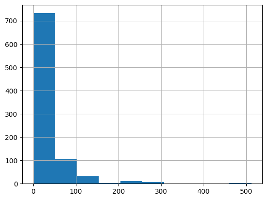
<Figure size 640x480 with 1 Axes>train_df["Fare"] = np.log(train_df["Fare"]+1)
train_df["Fare"].hist()
print("We now have a nicer distribution that will be easier to work with.")We now have a nicer distribution that will be easier to work with.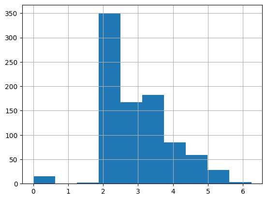
<Figure size 640x480 with 1 Axes>train_df.describe(include = [object]) Name Sex Ticket Cabin Embarked
count 891 891 891 891 891
unique 891 2 681 147 3
top Braund, Mr. Owen Harris male 347082 B96 B98 S
freq 1 577 7 691 646train_df = pd.get_dummies(train_df, columns=["Sex","Cabin","Embarked"],dtype=float)
train_df.head() PassengerId Survived Pclass \
0 1 0 3
1 2 1 1
2 3 1 3
3 4 1 1
4 5 0 3
Name Age SibSp Parch \
0 Braund, Mr. Owen Harris 22.0 1 0
1 Cumings, Mrs. John Bradley (Florence Briggs Th... 38.0 1 0
2 Heikkinen, Miss. Laina 26.0 0 0
3 Futrelle, Mrs. Jacques Heath (Lily May Peel) 35.0 1 0
4 Allen, Mr. William Henry 35.0 0 0
Ticket Fare Sex_female ... Cabin_F G73 Cabin_F2 \
0 A/5 21171 2.110213 0.0 ... 0.0 0.0
1 PC 17599 4.280593 1.0 ... 0.0 0.0
2 STON/O2. 3101282 2.188856 1.0 ... 0.0 0.0
3 113803 3.990834 1.0 ... 0.0 0.0
4 373450 2.202765 0.0 ... 0.0 0.0
Cabin_F33 Cabin_F38 Cabin_F4 Cabin_G6 Cabin_T Embarked_C Embarked_Q \
0 0.0 0.0 0.0 0.0 0.0 0.0 0.0
1 0.0 0.0 0.0 0.0 0.0 1.0 0.0
2 0.0 0.0 0.0 0.0 0.0 0.0 0.0
3 0.0 0.0 0.0 0.0 0.0 0.0 0.0
4 0.0 0.0 0.0 0.0 0.0 0.0 0.0
Embarked_S
0 1.0
1 0.0
2 1.0
3 1.0
4 1.0
[5 rows x 161 columns]We will remove the name attribute as it is not particularly useful for our predictions.
train_df = train_df.drop(columns=["Name","Ticket"])
train_df
PassengerId Survived Pclass Age SibSp Parch Fare Sex_female \
0 1 0 3 22.0 1 0 2.110213 0.0
1 2 1 1 38.0 1 0 4.280593 1.0
2 3 1 3 26.0 0 0 2.188856 1.0
3 4 1 1 35.0 1 0 3.990834 1.0
4 5 0 3 35.0 0 0 2.202765 0.0
.. ... ... ... ... ... ... ... ...
886 887 0 2 27.0 0 0 2.639057 0.0
887 888 1 1 19.0 0 0 3.433987 1.0
888 889 0 3 24.0 1 2 3.196630 1.0
889 890 1 1 26.0 0 0 3.433987 0.0
890 891 0 3 32.0 0 0 2.169054 0.0
Sex_male Cabin_A10 ... Cabin_F G73 Cabin_F2 Cabin_F33 Cabin_F38 \
0 1.0 0.0 ... 0.0 0.0 0.0 0.0
1 0.0 0.0 ... 0.0 0.0 0.0 0.0
2 0.0 0.0 ... 0.0 0.0 0.0 0.0
3 0.0 0.0 ... 0.0 0.0 0.0 0.0
4 1.0 0.0 ... 0.0 0.0 0.0 0.0
.. ... ... ... ... ... ... ...
886 1.0 0.0 ... 0.0 0.0 0.0 0.0
887 0.0 0.0 ... 0.0 0.0 0.0 0.0
888 0.0 0.0 ... 0.0 0.0 0.0 0.0
889 1.0 0.0 ... 0.0 0.0 0.0 0.0
890 1.0 0.0 ... 0.0 0.0 0.0 0.0
Cabin_F4 Cabin_G6 Cabin_T Embarked_C Embarked_Q Embarked_S
0 0.0 0.0 0.0 0.0 0.0 1.0
1 0.0 0.0 0.0 1.0 0.0 0.0
2 0.0 0.0 0.0 0.0 0.0 1.0
3 0.0 0.0 0.0 0.0 0.0 1.0
4 0.0 0.0 0.0 0.0 0.0 1.0
.. ... ... ... ... ... ...
886 0.0 0.0 0.0 0.0 0.0 1.0
887 0.0 0.0 0.0 0.0 0.0 1.0
888 0.0 0.0 0.0 0.0 0.0 1.0
889 0.0 0.0 0.0 1.0 0.0 0.0
890 0.0 0.0 0.0 0.0 1.0 0.0
[891 rows x 159 columns]import torch
from torch import tensor
labels = tensor(train_df['Survived'], dtype = torch.long)
attributes = tensor(train_df.drop(columns=['Survived']).values, dtype= torch.float)
label_atts_map = list(zip(attributes, labels))from torch.utils.data import random_split, DataLoader
train_size = int(len(label_atts_map)*0.8)
val_size = len(label_atts_map) - train_size
train, valid = random_split(label_atts_map, [train_size, val_size])
train_dl = DataLoader(train, batch_size = 64, shuffle = True)
valid_dl = DataLoader(train, batch_size = 64, shuffle = True)xb, yb = next(iter(train_dl))
yb.shapetorch.Size([64])import torch.nn as nn
import torch.optim as opt
model = nn.Sequential(
nn.Linear(1*158,512),
nn.ReLU(),
nn.Linear(512,256),
nn.ReLU(),
nn.Linear(256, 2),
)
learning_rate = 0.1
sgd = opt.SGD(model.parameters(), learning_rate)
loss_fn = nn.CrossEntropyLoss()print("Parameters shape: ", next(model.parameters()).shape)Parameters shape: torch.Size([512, 158])def validation():
accuracy = []
for xb, yb in valid_dl:
predictions = torch.argmax(model(xb))
accuracy.append((predictions == yb).float().mean())
return round(torch.stack(accuracy).float().mean().item(),4)
def train_epoch():
epoch_loss = np.array([])
for xb, yb in train_dl:
sgd.zero_grad()
predictions = model(xb)
loss = loss_fn(predictions, yb)
loss.backward()
epoch_loss = np.append(epoch_loss, loss.item())
sgd.step()
return epoch_loss
for ep in range(10):
mean_loss = round(np.mean(train_epoch()),4)
accuracy = round(validation(),4)
print(f"Epoch #{ep} || Mean Loss: {round(mean_loss,3)} || Accuracy: {round(accuracy,3)}")Epoch #0 || Mean Loss: 6.036624138778486e+18 || Accuracy: 0.6276
Epoch #1 || Mean Loss: 4.1381 || Accuracy: 0.6185
Epoch #2 || Mean Loss: 0.6586 || Accuracy: 0.6185
Epoch #3 || Mean Loss: 0.6694 || Accuracy: 0.6367
Epoch #4 || Mean Loss: 0.6694 || Accuracy: 0.6185
Epoch #5 || Mean Loss: 0.6695 || Accuracy: 0.6185
Epoch #6 || Mean Loss: 0.6613 || Accuracy: 0.6094
Epoch #7 || Mean Loss: 0.6563 || Accuracy: 0.5911
Epoch #8 || Mean Loss: 0.6651 || Accuracy: 0.6276
Epoch #9 || Mean Loss: 0.6698 || Accuracy: 0.6185Random Forests
Decision Trees
We will be building our decision tree using the sklearn library. Sklearn (also stylized as scikit-learn) is a Python library that is provides an API to easily create machine learning models.
Decision Trees try to split our dataset recursively until we reach a stop condition. The Decision Tree decides to make its splits in the following way.
- Go through each column in our dataset
- For each column, go through each possible level in that column (choose each possible value in that column)
- Try splitting the data into two groups based on each level (our binary split)
- Find the average value of the target for both groups.
- Compare this average value to the actual target value for each individual in each group.
- After looping through all of the columns and all of the possible levels in each column, choose the split that provided the best prediction found in the previous step.
- Repeat this process with our two subgroups. Stop until we reach our stop condition (ie max depth, min number of individuals per group).
Preprocessing our data
Similarly to our neural network, we need to preprocess our data before being able to use it for our model.
train_df = pd.read_csv("./titanic/train.csv")
train_df
PassengerId Survived Pclass \
0 1 0 3
1 2 1 1
2 3 1 3
3 4 1 1
4 5 0 3
.. ... ... ...
886 887 0 2
887 888 1 1
888 889 0 3
889 890 1 1
890 891 0 3
Name Sex Age SibSp \
0 Braund, Mr. Owen Harris male 22.0 1
1 Cumings, Mrs. John Bradley (Florence Briggs Th... female 38.0 1
2 Heikkinen, Miss. Laina female 26.0 0
3 Futrelle, Mrs. Jacques Heath (Lily May Peel) female 35.0 1
4 Allen, Mr. William Henry male 35.0 0
.. ... ... ... ...
886 Montvila, Rev. Juozas male 27.0 0
887 Graham, Miss. Margaret Edith female 19.0 0
888 Johnston, Miss. Catherine Helen "Carrie" female NaN 1
889 Behr, Mr. Karl Howell male 26.0 0
890 Dooley, Mr. Patrick male 32.0 0
Parch Ticket Fare Cabin Embarked
0 0 A/5 21171 7.2500 NaN S
1 0 PC 17599 71.2833 C85 C
2 0 STON/O2. 3101282 7.9250 NaN S
3 0 113803 53.1000 C123 S
4 0 373450 8.0500 NaN S
.. ... ... ... ... ...
886 0 211536 13.0000 NaN S
887 0 112053 30.0000 B42 S
888 2 W./C. 6607 23.4500 NaN S
889 0 111369 30.0000 C148 C
890 0 370376 7.7500 NaN Q
[891 rows x 12 columns]def proc_data(df):
df['Fare'] = df['Fare'].fillna(0)
df.fillna(modes, inplace=True)
df['LogFare'] = np.log1p(df['Fare'])
df['Embarked'] = pd.Categorical(df['Embarked'])
df['Sex'] = pd.Categorical(df['Sex'])
proc_data(train_df)The pd.Categorical method will replace in the background the categorical variable with a code.
Let us now define our categorical and continuous variables that will be of interest and replace our categorical variables with their code.
categoricals = ['Sex', 'Embarked']
continous = ['Age', 'SibSp', 'Parch', 'LogFare', 'Pclass']

dependent = 'Survived'

train_df[categoricals] = train_df[categoricals].apply(lambda x: x.cat.codes)
from numpy import random
from sklearn.model_selection import train_test_split
random.seed(42) # define our random seed to help make this repeatable
trn_df, val_df = train_test_split(train_df, test_size = 0.25)
def split_target_input(df):
xs = df[categoricals+continous].copy()
return xs, df[dependent]
trn_xs, trn_y = split_target_input(trn_df)
val_xs, val_y = split_target_input(val_df)Training Our Decision Tree
from sklearn.tree import DecisionTreeClassifier, plot_tree

tree = DecisionTreeClassifier(max_leaf_nodes = 4).fit(trn_xs, trn_y)
plot_tree(tree, feature_names = trn_xs.columns, filled=True)
print("A graph of our decision tree")A graph of our decision tree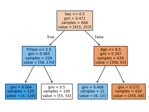
<Figure size 640x480 with 1 Axes>The giniscore is a measure of the impurity of our groups. The lower the gini the more dissimilar each individual in each group is.
#Our metrics function
def mean_square_error(predictions, targets):
    return np.mean((predictions-targets)**2).item()
mean_square_error(tree.predict(val_xs), val_y)0.2242152466367713Bagging + Random Forests
Bagging is a technique developed by Leo Breiman (a UC Berkeley professor; go bears!) that consists of taking a bunch of different models that are trained on bootstraps of our data (random selections of our training data). We then use each model to make a prediction and then take the average of those predictions.
The idea behind this method is that each model is independent of each other. Therefore there errors will be independent of each other and when averaged out they should tend to zero.
A great feature of random forests is that it is not possible to overfit a random forest as each model is independent of each other.
A random forest is the bagging of decision trees. Random Forests and Bagging more generally are an example of ensembling.
# A function that defines a bootstrapped tree

def get_tree(prop=0.75):
    length = len(trn_y)
    idxs = random.choice(length, int(length*prop)) # returns random indices to look at
    return DecisionTreeClassifier(min_samples_leaf = 5).fit(trn_xs.iloc[idxs], trn_y.iloc[idxs])
def random_forest(xs, length=100):
preds = np.stack([get_tree().predict(xs) for _ in np.arange(length)])
return np.mean(preds, 0)preds = random_forest(val_xs)
mean_square_error(preds, val_y)0.13712600896860988# using sklearn
from sklearn.ensemble import RandomForestClassifier
rf = RandomForestClassifier(100, min_samples_leaf = 5)
rf.fit(trn_xs, trn_y)
mean_square_error(rf.predict(val_xs), val_y)0.18385650224215247title = "Feature importance of our random forest model"
plt = pd.DataFrame(dict(cols=trn_xs.columns, imp=rf.feature_importances_)).plot('cols', 'imp', 'barh', title = title)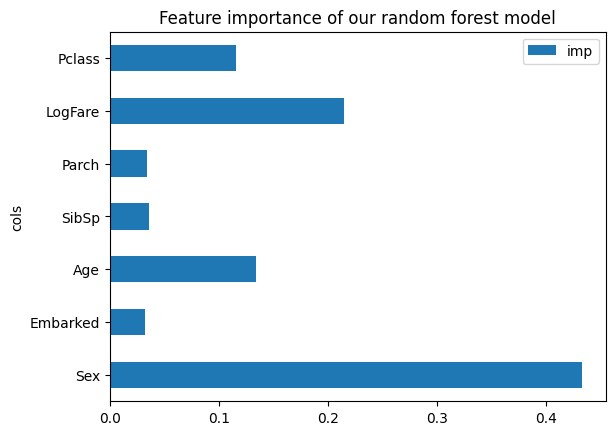
<Figure size 640x480 with 1 Axes>Here above is one of the great features of Decision Trees / Random Forests. We are able to see the relative importance of each feature in making a prediction.
Gradient Boosting Machine
This is another type of ensembling technique for random forests. Instead of averaging out the predicitons, each prediction is summed. This is called boosting.
Gradient Boosting Machine are prone to overfitting apparently for no apparently reason.